Outperforming the Market Using a Forward P/E Moving Average Strategy.

The stock market can be a volatile and confusing place, but with the right strategy, investors can maximize their returns. In this article, I present the Moving Average P/E Switch, which uses the moving average of the (Bloomberg) estimate of the P/E (price-to-earnings) ratio for the next 12 months to determine whether to invest in value stocks or growth. Specifically, I use the SPDR SPYV to represent value and SPDR SPYG to represent growth. In theory, one of the measures of relative valuation might help predict a value or growth bias, but I have not seen it applied anywhere else. So, for the time being, this strategy remains proprietary and will not be published.

This article will break down the Moving Average P/E Switch strategy step by step, I will also attach the commented code at the end.

Finding the Relationship

Companies in the S&P 500 are valued for their earning potential over time. Growth stocks, those that derive value from future cash flows, are contrasted with value stocks, which derive value from current operations.

The P/E ratio measures relative valuation and is a common tool used to determine if a company is overpriced or underpriced. Companies with a “growth” bias, have a higher relative valuation. In contrast, companies with a lower relative valuation, have a “value” bias. This does not always hold but it is generally accepted.

Based on this information, we can use the P/E of the market to assess whether there’s a value or growth bias in the market and pick between them. If relative valuations are high, or, better put, if relative valuations are increasing, we will choose Growth. Analogously, if relative valuations are decreasing, we will choose Value.

The data

To find the degree of this relationship, I downloaded data and plotted a correlation matrix. The date ranges from the start of the century until today. The variables I used are the following, I also calculated the daily return for each of these variables. (I also tried with EPS, Best EPS, Sales, and Best Sales, but no relevant relationship was found.)

• P/E: The current market Price to Earnings Ratio
• Best P/E: The Bloomberg estimate of the P/E ratio for the next 12 months.
• SPY: SPDR S&P 500 ETF Trust (SPY) Prices.
• SPYV: SPDR Portfolio S&P 500 Value ETF Prices.
• SPYG: SPDR Portfolio S&P 500 Growth ETF Prices.

Imported Data looks like this

Let’s start with the code:

#Import Packagesimport pandas as pdimport scipy.optimize as optimport matplotlib.pyplot as pltimport seaborn as snsimport numpy as npimport quantstats as qs #Import Data // change "path" to your pathdf = pd.read_excel(r"path")df = df.set_index('Date')df = df.loc[df.index >= '2001-04-11']# Calculate percent changesdf['PE_CHANGE'] = df['PE'].pct_change()df['BEST_PE_CHANGE'] = df['BEST PE'].pct_change() df['SPY_RETURNS'] = df['SPY'].pct_change()df['SPYV_RETURNS'] = df['SPYV'].pct_change()df['SPYG_RETURNS'] = df['SPYG'].pct_change()#Show the correlation matrixdf.corr()

Press enter or click to view image in full sizeCorrelation Matrix

Based on this information, it’s worth giving it a try.

2. Developing the strategy.

In this part, we need to measure how the BEst P/E is changing. To do this, we use the 20-day moving average of the change. If it is above 0, the BEst P/E is increasing, which means forward relative valuation is increasing, so we should pick Growth. If the moving average is below 0, the opposite logic applies, so we should pick Value. Instead of determining whether the moving average is negative or positive, we can compare it to the historical average, which would turn out to be a measure of relative change in the market’s expectation of relative valuation. (In the code, we actually optimize to find the threshold that results in the best historical returns). Based on the results of the optimization, if the 20-day moving average of the change in the BEst P/E ratio is less than 0.00010109.

# Calculate moving averagedf['BEST_PE_CHANGE_MA20'] = df['BEST_PE_CHANGE'].rolling(window=20).mean()# Define function to optimizedef strategy_returns(threshold, df): df['RETURNS'] = df.apply(lambda x: x['SPYV_RETURNS'] if x['BEST_PE_CHANGE_MA30'] < threshold else x['SPYG_RETURNS'], axis=1) #Create final value of cumulative investment strategy_investment = 100 * (1 + df['RETURNS']).cumprod() return -1*strategy_investment.iloc[-1] # minimize negative of final value# Define boundsbnds = ((0.00010000, 0.00020000),)# Initial threshold guessx0 = [0.0001000]# Maximize the functionres = opt.minimize(strategy_returns, x0, args=(df,), bounds=bnds, method='SLSQP', options={'disp':True, 'maxiter':1000})# Extract the optimal thresholdoptimal_threshold = res.x[0]print(optimal_threshold)#optimal threshold is 0.00010109#Create a "RETURNS" column that chooses value or growth according to the conditions explaineddf['RETURNS'] = df.apply(lambda x: x['SPYV_RETURNS'] if x['BEST_PE_CHANGE_MA30'] < optimal_threshold else x['SPYG_RETURNS'], axis=1)

In summary:

• Best P/E ⬇️ → Value
• Best P/E ⬆️ → Growth
• ΔBest P/E < 0 → Value
• ΔBest P/E > 0 → Growth
• MA(20)ΔBest P/E < 0.00010109 → Value
• MA(20)ΔBest P/E > 0.00010109 → Growth

3. Results and Backtesting

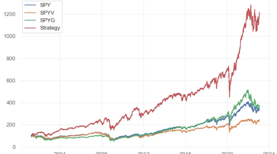
#Calculate cumulative returnsspy_investment = 100 * (1 + df['SPY_RETURNS']).cumprod()spyv_investment = 100 * (1 + df['SPYV_RETURNS']).cumprod()spyg_investment = 100 * (1 + df['SPYG_RETURNS']).cumprod()strategy_investment = 100 * (1 + df['RETURNS']).cumprod()# Print final valuesprint("Value of $100 investment in SPY:", spy_investment.iloc[-1])print("Value of $100 investment in SPYV:", spyv_investment.iloc[-1])print("Value of $100 investment in SPYG:", spyg_investment.iloc[-1])print("Value of $100 investment in Strategy:", strategy_investment.iloc[-1])#Plot using matplotlib#Graphsplt.plot(spy_investment, label='SPY')plt.plot(spyv_investment, label='SPYV')plt.plot(spyg_investment, label='SPYG')plt.plot(strategy_investment, label='Strategy')plt.legend()plt.show()#Plotting the returnsplt.plot(df.index, df['SPY_RETURNS'], label='SPY')plt.plot(df.index, df['SPYV_RETURNS'], label='SPYV')plt.plot(df.index, df['SPYG_RETURNS'], label='SPYG')plt.plot(df.index, df['RETURNS'], label='Strategy')plt.legend()plt.show()#Use quantstats package for backtesting report that returns some of the images provided below. #Once again replace path with your own path. metrics = qs.reports.html(df['RETURNS'], df['SPY_RETURNS'], start='2001-01-01', end='2022-12-31', mode='full', output=r"C:\Users\path\quantstats-tearsheet.html")

The strategy chooses Growth about 55% of the time.

The moving average of the P/E estimate for the next 12 months is a simple yet effective tool for switching between value and growth biases. The implementation of this strategy, as outlined in this article, can provide a roadmap for investors looking to optimize their investments and achieve their financial goals.

The information provided in this article is for informational purposes only and should not be considered financial or investment advice. The author and any associated parties make no representations or warranties as to the accuracy or completeness of the information contained in this article. The information provided is not a recommendation to buy or sell any security or engage in any particular investment strategy. The author and any associated parties will not be liable for any direct, indirect, incidental, or consequential damages resulting from the use of this information.